
Embarking on a demand-driven journey can require a leap of faith, trusting a new way of planning and executing replenishment processes to ensure realization of customer service and inventory goals.
That’s what demand-drive replenishment (DDMRP) does, and understanding the theory behind it helps you gain confidence in the success of practice.
But there are still those nagging doubts, at least if you’re like me, particularly as one who has spent over 30 years working with traditional MRP systems.
In those systems, it’s simple to create a demand forecast for parent level items as far in the future as needed and see what happens from a materials and capacity perspective. That’s pretty much what master production scheduling is!
DDMRP does not necessarily offer this capability. While average daily usage (ADU) and buffer sizes can be calculated in the future, as SAP Integrated Business Planning (SAP IBP) for demand-driven replenishment does, the evaluation of net flow position (NFP) and generation of supply orders happens daily. And it happens at decoupling points where demand pull from either customer or dependent demand is based on orders, not explosion of a bill of materials or bill of distribution to drive planned demand. Once you’re live with DDMRP, that’s fine—the processes inherent in the five step model will keep supply and demand synchronized as intended.
We all agree, right? I hope so, but also understand a little skepticism. I often tell customers that the toughest part of any DDMRP project is not the technical side, but the process side. Wouldn’t it be great if there were a simple way to model the future under a DDMRP environment?
With SAP IBP, there is. In my recent SAP PRESS E-Bite Introducing DDMRP with SAP IBP, I mention briefly an SAP IBP parameter called “current period offset.” Defined at the header level of each planning area, this small but powerful value tells the planning area what the current date is. Ordinarily it is not noticed, with the value set to 0, indicating that the current date is today (as it should be). Most business users of SAP IBP may not be aware of its existence—here’s what it looks like.
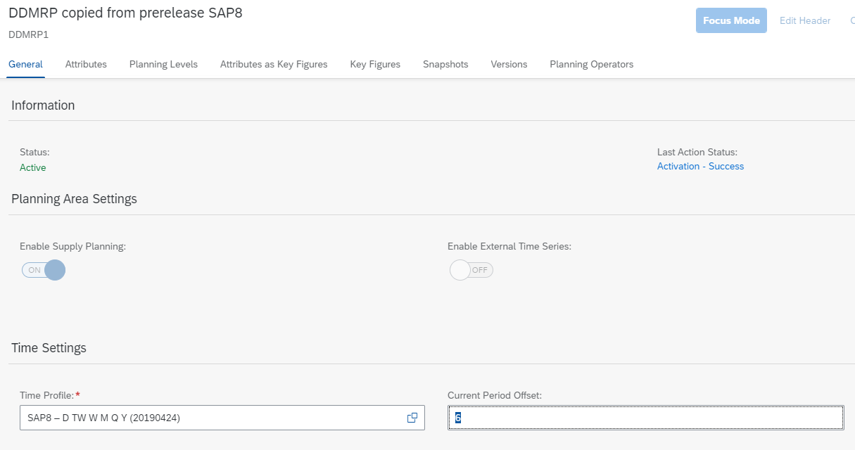
Educators, implementers, and those of us who demonstrate the product certainly are familiar with this—it’s invaluable in testing and showing capabilities. (Less so when working with time series IBP, where past and future horizons may be specified. For DDMRP, it’s always “today.”)
If you’ve been educated in DDMRP you know that the set of “Day 0->Day 1->Day n” examples are critical to building understanding of how NFP is calculated and supply orders are generated.
If you’ve tried to do this yourself, you know that some Microsoft Excel skill is required, and there is a direct correlation between Excel skill/investment in build time and ease of advancing from day to day. This is not necessarily a bad thing in a simple case, as it builds a deeper understanding of the algebra that makes DDMRP work and is a valid part of DDMRP education.
Nonetheless, that doesn’t help when you’re seeking to assess the performance of your company’s actual DDMRP model.
Successive iterations of SAP IBP for demand-driven replenishment, with changes to the Current Period Offset parameter between each, can.
Here’s a basic process:
Setup
Have your master data set and ready to test. Pay particular attention to the settings that determine ADU calculation (forward and backward horizon) and buffer sizing. Then pick a set of relevant decoupling points to test.
You can load real or simulated demand, in the past, and—if using forward-looking ADU—in the future. Using Excel’s RANDBETWEEN() function as in input to further calculation makes this simple. If you’re testing decoupling points with dependencies, remember that SAP IBP will not be calculating dependent demand in the ADU determination process. When creating demand for child location/products, either set the appropriate seed value for the RANDBETWEEN() or model the quantity per assembly in an Excel formula based on the parent. (I usually do the latter, and put a RANDBETWEEN() after the base calculation to introduce variability.) The range of the RANDBETWEEN() parameters will impact the variability of the demand stream, and perhaps the variability category used in buffer sizing.
Execute and review the ADU and buffer size planning operators. Make sure the results are as expected; if not, determine why and make the appropriate adjustments. Perhaps this is due to forward and backward horizons, or buffer determination settings.
For materials that are at the top-level decoupling point—that is, driven by either customer demand or demand from a non-DDMRP parent—save future values of confirmed demand order quantity for the horizon you’re going to test. If you calculated ADU with a forward looking horizon, you could just copy the values already used. If not, use RANDBETWEEN() as in the step above to load future demand.
Note that demand generated on this basis will fall below the spike threshold, and will thus influence NFP calculation only when present in the current or prior periods. If you want to include spike demand in your testing, feel free. Either use a broader RANDBETWEEN() range or manually drop in spikes.
Materials where demand is dependent on parent DDMRP planned items included in the test will be handled separately.
Testing (Iterative)
Set the current period offset (CPO) to a NEGATIVE value greater than or equal to the longest decoupled lead time (DLT) of the materials being tested and review the NFP in Excel.
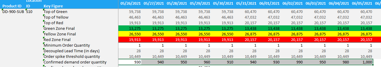
Fabricate on-hand inventory and open supply such that the NFP status is in the bottom of green (no order needed). Set the CPO one week ahead. You could do daily, as in real life, but for the purposes of this testing weekly is generally sufficient. Then evaluate the new NFP. Below explores the manual parts of each iteration.
For each material, if a new supply order is recommended, place its quantity as a confirmed supply order quantity value in the column to the right that corresponds to its decoupled lead time.
If the demand element created will drive demand for other items in the test, create a confirmed demand order quantity for these materials n columns to the left of the parent supply order, where n is the parent items production or transport lead time. One could debate whether the preceding step should be done before or after calculating NFP of the child material. If iterating this process daily, then you should definitely choose after. If weekly, after is still simpler, recognizing that your test may penetrate child material buffers more deeply than otherwise due to a one week latency in order placement.
Calculate on-hand inventory into the future using Excel to add the prior day’s on-hand to current day supply, less current day demand. Copy this formula at minimum as far into the future as your iteration period (i.e. weekly). Save the contents of your Excel view, then delete the values of confirmed supply and demand orders in the current and any preceding periods (i.e. with a weekly iteration, for the past week). Save again.
That completes a one-week cycle. Now, add the number of days in one iteration to the CPO, save, and refresh the Excel view. Time will have passed, and a new NFP will be calculated and shown. Since we started this in the past, the appropriate on-hand inventory and supply elements will be loaded at the actual start date of the test. Alternatively you can make up the data to have the actual start appear in the high yellow or low green. With short DLT materials, this would work fine.
Note that as you repeat this process and calculate on-hand inventory per the process above, you will be creating each day’s inventory and saving past values—this will be important at the end of the test. SAP IBP for demand-driven replenishment does this to the calculation, but in the standard planning area it uses ADU rather than actual demand. You may choose to change the definition and use this key figure instead.
Continue this iterative process through the test period. At each iteration, in addition to reviewing NFP and creating demand and supply orders, assess the projected on-hand inventory for one DLT out of each material. If you have a week’s latency in creating supply, you may see deeper penetration into the red than you’d like, but understand this is a function of the test.
Important—if you see any projected stockouts, ensure the team understands why, and what changes might be made to prevent this. But that’s a topic beyond the scope of this post. That said, if the stockout period is less than a week, don’t be too concerned. Daily iteration would have placed a supply order earlier and mitigated that.
You are always free to change from weekly to daily cycles. This can be particularly important if you are testing materials with cyclical or seasonal demand.
Continue this process until the end of the test period.
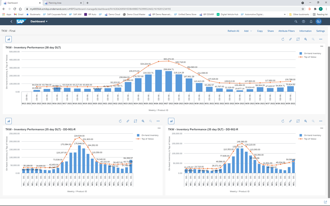
I recently ran this process for a 180-day period for three materials, and it took less than an hour. When complete, I was able to assess overall performance (Note that the business basis of this test will be discussed in a separate post.)
You’ll note that this process is not fully automated… so you will want to manage the scope of your testing exercise. I used materials that did not have dependent demand from another DDMRP part, which reduces the effort required (see above where I talk about the relationship between supply elements for a parent item and demand for the child). Do just enough to convince yourself, and the skeptics on your team, that DDMRP will perform as you expect.
Also, when used in an internal education, rather than testing, for context make sure to add exploration of the relevant KPI’s in Excel and the web UI (particularly custom alerts) to understand the feedback your team will receive, and the actions thus taken.
Finally, this exercise does not leverage the SAP ECC integration that you will use in the product for the simple reason that as far as SAP ECC is concerned, today is today. So we just fake it.
Conclusion
That’s all there is to it! Please keep in mind that the full simulation capabilities of SAP IBP are behind this—alternative versions were used to assess different master data with the same demand, and simulations introduced greater variability and spikes into the demand stream to test buffer resilience. Comprehensive testing enables confidence in the results to be achieved in production, and the test results may even be saved for assessment against actuals as you go live.


Comments