
If you’ve ever faced the challenge of planning the production of variant configured products beyond the customer order horizon, you know the challenges and pitfalls that make this one of manufacturing’s toughest problems.
Within the horizon, SAP does this exceptionally well with either production planning and detailed scheduling (PP-DS), or, more appropriately, model mix planning/sequencing. This can be done because the system already has customer orders for specific configurations and associated manufacturing orders calling out the bill of materials (BOM) and routing elements needed to plan.
Beyond the horizon, not so much. Planning at an aggregate level (how many snowmobiles, or tractors, or trucks...?) is well supported. The challenge is planning for selectable features and options, and the associated materials and resource requirements.
The ERP industry—including SAP—has done the best that can be done with the use of planning bills, which use an attach rate model to express component requirements as a percentage of parent item demand. SAP ECC, SAP S/4HANA, and SAP Integrated Business Planning (SAP IBP) all support this.
Limitations of Current Planning Models
You don’t have to think too long about this to see the issue—this process does not respect any dependencies among the selections. For example, I may say 1600cc engines and 2400cc engines have attach rates of 60% and 40% respectively. And six-speed and four-speed transmissions are 50%/50%. But if I can only use the six-speed with a 2400cc engine, that rule cannot be comprehended and the results will be less than fully accurate.
Going any further is one of the most difficult computer science problems in supply chain. Google shows no good answers. To do this right, you need to be forecasting future orders using the full variant configuration (VC) model, with parameter driven inputs. And, likely, some Monte Carlo analysis thrown in to account for variability. If you come even close to getting that right, good luck with forecast consumption. If SAP’s engineers, and its competitors, have not been able to develop a comprehensive solution, you can bet it’s just pretty darn hard to do.
Which does not prevent planners the world over from having to do something, as it’s the nature of their business.
Demand-Driven MRP
For them, and perhaps for you, good news! And good news that comes via a simple, elegant solution—demand-driven MRP (DDMRP). You may be familiar with the concept; if not, a comprehensive discussion is beyond the scope of this blog. See the Demand Driven Institute for more information.
For our purposes here, let me just state the most basic of DDMRP principles: When customers demand product, configured or otherwise, be delivered in less than the cumulative lead time required to procure materials and perform the necessary production and transportation steps, buffer inventory must be maintained to shorten the lead time.
Nothing new here. What’s new in DDMRP is the art and science associated with determining which materials, and where, to set as “strategic decoupling points,” and the process by which appropriate buffer sizes are calculated and material flow ensured based on demand pull. SAP delivers these capabilities, and more, in both SAP S/4HANA and SAP IBP for demand-driven replenishment. For more information on the SAP IBP solution, please see my recent SAP PRESS E-Bite.
While DDMRP is not just, or even specifically, for organizations whose end products are made-to-order or assemble-to-order with VC, its principles and implementation uniquely provide a solution to this difficult problem.
Here’s how. In a simple example, let’s assume we’re a powersports company making a line of personal watercraft with the option of a 1600cc or 2400cc engine. With everything else being standard, we can assemble a watercraft in one day. But the engines take six weeks to arrive. In the past, we’ve been able to use a planning bill, specifying the engines as a fractional quantity per assembly sometimes called an attach rate. For example, 60% of our watercraft get a 1600cc engine, 40% a 2400cc. If we stopped there, we would not have a problem worth writing about. Our current practices are likely adequate. But the real world is not that simple; there are likely other optional components involved, at multiple BOM levels, and dependency rules governing their selection. Dependencies, in particular, break the attach rate model quickly, and render standard planning tools less that ideal.
So let’s change the game. If we understand the BOM and supply network associated with the end item, and the lead time of each step, DDMRP theory enables determination of where strategic decoupling points should be placed to ensure that the decoupled lead time (the time to produce based on final assembly, plus the time from the longest-feeding supply chain) is less than the customer’s tolerance time. SAP IBP for demand-driven replenishment does this calculation explicitly.
In the simple example we’re talking about, it’s a safe bet that each engine would be identified as a decoupling point just due to lead time. There may be others in the network as well. For each material/location decoupling point, we know the historical demand; from this, the average daily usage of the material and the variability of this variable can be calculated. These and other values, along with the decoupled lead time of the material, enable calculation of the appropriate inventory buffer sizes. While the algebra is simple, real world scale requires software like SAP IBP to support the analyst.
Once the buffers have been calculated, DDMRP uses demand and supply to calculate an availability measure called the net flow position (NFP), and the value of the NFP is relative to the buffer sizes to determine when supply elements are required—entirely on a pull basis.
In our watercraft example, we can stop using attach rate planning and let the demand signals processed by DDMRP ensure that we have sufficient engines on hand to support final assembly. Other components—particularly those used 100% as part of the base product—may well still be planned with traditional MRP. (Though it’s likely that many will also be identified as decoupling points.)
Simple, isn’t it? And elegant and intuitive as the concept expands on what most are already doing in practice with other tools.
Possible Objections and Answers to DDMRP
And right about here, someone will throw one of several valid objections, including:
- We often have product supersession planned at future dates. How does this model handle that?
- Our production is highly cyclical, and we don’t build watercraft all year. How do we ensure availability as production ramps up?
All of the objections have a common root cause—DDMRP as we’ve discussed it so far assumes demand for a product, while variable, will vary around a relative stable mean. The concerns above result from a situation where this is false.
Fortunately, DDMRP theory, and SAP’s implementation of it, provide an answer here too. Though it does involve a forecast.
The forecast is used to adapt the calculation of average daily usage by specifying the number of periods (forwards and backwards) used. Default is all backwards; the results are analogous to a moving average, albeit one that does not look beyond today.
For a newly introduced product, using only future forecasting would be appropriate, allowing buffer sizes to adapt as demand increases and then stabilizes. The same is true in the case of material supersession, where the old material will see usage decreasing to zero, and the new one ramping up.
A “blended average daily use,” with forward and backward periods, serves to consume and consider a forecast while dampening its immediate impact.
By using this capability, we can enable DDMRP to plan effectively with unstable demand streams.
But there is one very important consideration. Traditional MRP generates dependent demand based on a BOM relationship and uses this to drive lower level material requirements. The presence of decoupling points in DDMRP limits the applicability of this logic, instead requiring a forecast of each buffered part independent of its parent material(s).
This means you have two options to generate a forecast for these buffered materials:
- Statistical forecast using a univariate or multivariate model. This may be valid for materials that have been consistently part of the feature set over time, and have had relatively stable attach rates.
- Explosion via attach rates and a planning BOM. Yes, I know we discounted this earlier. But that was as a driver for deterministic MRP. In this context, it’s the only way to deal with three “real world” considerations:
- Attach rates are expected to differ in the future
- New product introduction or supersession change the component required
- Demand for the parent item(s) is expected to differ from the past.
If any of these characteristics are present, a statistical forecast at the item level may not be sufficient. Fortunately, as we’ve also already noted, the attach rate forecast is easy to obtain through the SAP IBP supply heuristic.
As is the case in determining consensus demand in a basic S&OP cycle, we recommend doing both—statistical and attach rate—and comparing the results. Significant differences should be understood and a decision made on the final forecast.
For this test case, we’ve created a significant cyclical demand case, which is reflected in our future forecast and the associated average daily use (ADU).
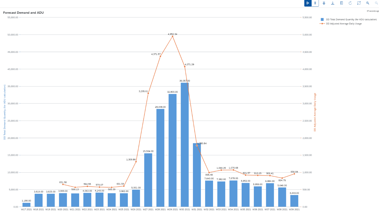
Once you have a forecast, SAP IBP takes over and calculates average daily usage and, subsequently buffer sizing. This is the science part. The “art,” and something you may choose to explore further, are the forward and backward horizons. Building on the issues introduced earlier:
- Shorter horizons lead to a more “nervous” average daily use, which is not ideal but may be required.
- A longer backward horizon makes average daily use changes less responsive to changes in the future, slowing the increase or decrease in buffer size. When ramp or ramp down is rapid, as in the NPI scenario discussed earlier, you may choose zero backward
- The forward horizon should start as (at least) one decoupled lead time. Any less, and insufficient stock may be on hand as demand increases.
Then…turn it on. Well, maybe not. This sounds a little too simple, perhaps?
Testing Your Forecasts
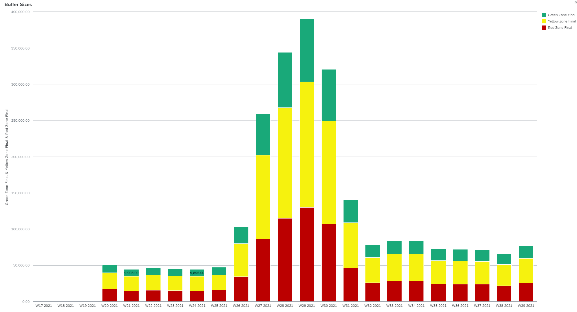
Fortunately, SAP IBP provides a facility for some testing using a parameter called the current period offset, which allows you to simulate the passage of time. This is critical with a process like DDMRP, which assesses the NFP and reacts daily. I’ve covered this testing process in a separate post (“Testing a DDMRP Model with SAP IBP for Demand-Driven Replenishment”) in which I tested just the case described here. As you’d expect from the ADU, the buffer sizes are also cyclical.
We’ve addressed creating appropriately sized buffers, but what about the lead time issue? Fortunately, SAP IBP for demand-driven replenishment takes care of that too. In a slight (but approved, and important) departure from basic DDMRP theory, SAP IBP evaluates the net flow position one decoupled lead time in the future. This ensures that pending increases in buffer size are recognized and planned in time to secure materials, so that upon receipt the quantity on hand is consistent with the then-current buffers.
Please understand that this was not a rigorous academic test using discrete event simulation. I actually found many of these on the web; Google “discrete event simulation DDMRP” and you will too.
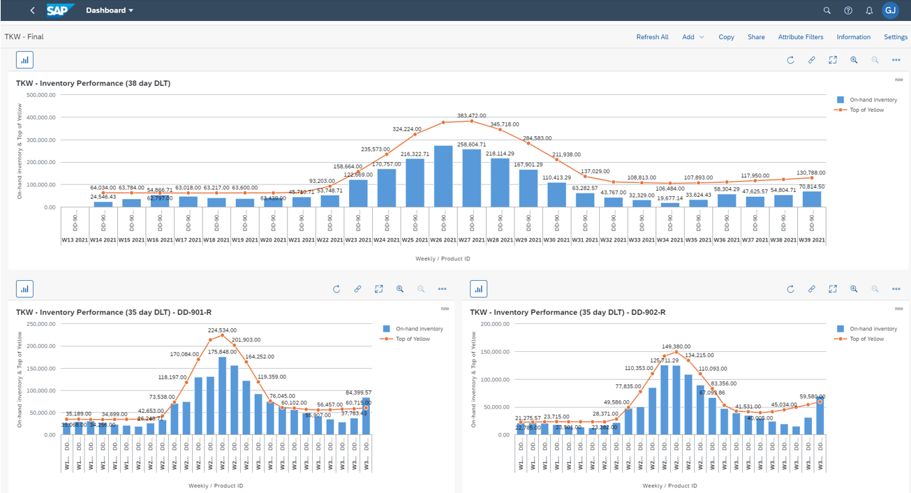
But I did simulate a 180-day cycle with a significant demand increase in the middle, where the end item was MRP planned (and therefore not in the test) and three key components were DDMRP planned.
The results suggest that DDMRP does adequately support this use case, with DDMRP inventory tracking demand as expected.
Are we still exposed? Of course. Our planning here is forecast driven, and forecasts are wrong. But DDMRP—through the explicit use of buffers—provides a more robust capability to absorb variation than deterministic MRP. The test case I ran did not include any real-time course correction—for example, using SAP IBP demand sensing to assess differences between actual and forecast demand, or even reforecasting during the execution period.
We have not “proven” anything, necessarily. But the results of this test do support confidence in the ability of DDMRP to support planning for configured materials effectively.


Comments